Fast Multipole Acceleration

FMM accelerates Green’s function interactions of the form

\[ u(x_j) \approx \sum_{i=1}^N G(x_j,y_i)\,s_i, \qquad j=1,\dots,M. \]

Forming the complete interaction matrix requires \(O(MN)\) storage, while direct evaluation of the sum costs \(O(MN)\) operations.

The fast multipole method avoids treating all interactions equally. Nearby interactions are kept accurate and direct while far interactions are approximated by expansions around cluster centers.

Where FMM Enters BEM

For a scalar single layer operator, a Galerkin BEM matrix entry is

\[ A_{ij} = \langle V\varphi_j, \eta_i \rangle_\Gamma = \int_\Gamma \int_\Gamma \eta_i(x)\,G_\kappa(x,y)\,\varphi_j(y) \,d\sigma_y\,d\sigma_x. \]

After quadrature,

\[ A_{ij} \approx \sum_\alpha w_\alpha^x\eta_i(x_\alpha) \underbrace{ \sum_\beta G_\kappa(x_\alpha,y_\beta) \underbrace{w_\beta^y\varphi_j(y_\beta)}_{s_\beta^{(j)}} }_{\text{FMM source to target sum}}. \]

The inner sum has exactly the source to target form accelerated by FMM.

Near Field and Far Field

The FMM splits quadrature point interactions by cluster geometry:

• near field: boxes that are not well separated are evaluated directly using SIMD,

• far field: well separated boxes are evaluated using multipole and local expansions.

Touching boundary elements require an additional sparse BEM correction:

\[ A = A_{\mathrm{FMM}} + \left( A_{\mathrm{touch}}^{\mathrm{accurate}} - A_{\mathrm{touch}}^{\mathrm{quadrature}} \right). \]

The accurate entries use Sauter Schwab rules [SS09] based on Duffy transformations.

Regular and Singular Expansions

Following [GD04], the Helmholtz basis functions in spherical coordinates:

\[ R_n^m(x-c) = j_n(\kappa r)\,Y_n^m(\theta,\phi), \qquad S_n^m(x-c) = h_n^{(1)}(\kappa r)\,Y_n^m(\theta,\phi). \]

Here \(r=|x-c|\), \(Y_n^m\) are spherical harmonics, \(j_n\) are spherical Bessel functions, and \(h_n^{(1)} = j_n + i y_n\) are outgoing spherical Hankel functions.

Regular expansion:

\[ u_R(x) \approx \sum_{n=0}^{p-1}\sum_{m=-n}^{n} a_n^m R_n^m(x-c). \]

• finite at the expansion center,

• used for local target expansions.

Singular expansion:

\[ u_S(x) \approx \sum_{n=0}^{p-1}\sum_{m=-n}^{n} b_n^m S_n^m(x-c). \]

• singular at the expansion center,

• outgoing for Helmholtz; satisfies the Sommerfeld radiation condition,

• used to represent the field generated by a source cluster.

Bessel and Hankel Stability

The radial basis functions satisfy the recurrence

\[ f_{n+1}(z) = \frac{2n+1}{z} f_n(z) - f_{n-1}(z). \]

For small \(|z|\) and large \(n\), direct recurrence may overflow or underflow. NGSolve computes \(j_n\) backwards and rescales large intermediate values. A forward pass applies the accumulated scaling and normalizes the result. The functions \(y_n\) are then computed forwards and combined as \(h_n^{(1)}=j_n+i y_n\).

Multilevel FMM

Source and target points are grouped in an adaptive tree. The computation moves upward, across well separated boxes, and downward to the targets.

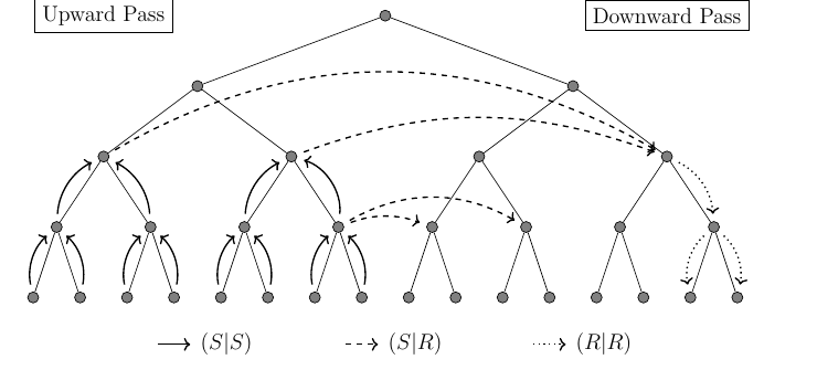
A translation in an arbitrary direction is split into three simpler steps:

1. rotate the coordinate system so the translation direction becomes the \(z\) axis,

2. translate along the \(z\) axis,

3. rotate back.

As a matrix product, this can be written in the form

\[ T(\ell,\theta,\phi) = D(-\phi)\,C(\ell,\theta)\,D(\phi), \qquad C(\ell,\theta) = Y(-\theta)\,A(\ell)\,Y(\theta). \]

Here \(A(\ell)\) translates along the \(z\) axis, \(Y\) changes the polar direction, and \(D(\phi)\) is a cheap azimuthal phase factor. The \(z\) axis translation preserves \(m\) and therefore has block structure. Applied directly, a translation couples all \(p^2\) input coefficients with all \(p^2\) output coefficients and costs \(O(p^4)\). Splitting it into rotations and a \(z\) axis translation reduces the cost to \(O(p^3)\).

Computing the entries of the \(z\) axis translation matrix \(A(\ell)\) accurately requires care with scaling and the order in which recurrence relations are evaluated [Dor25].

For stable computation of the matrix \(Y(\theta)\) representing rotation about the \(y\) axis, [GD15] presents recurrence relations for spherical harmonic rotation coefficients together with an analysis of their numerical stability. An overview of this construction is given in [Dor25].

For one source and target box pair, a normal translation is

\[ a^{\mathrm{out}} = T(\ell,\theta,\phi)a. \]

Here \(p\) is the expansion order, using degrees \(n=0,\dots,p-1\), so \(a \in \mathbb{C}^{p^2}\) contains \(p^2\) coefficients.

Within each translation type, the implementation groups \(q\) translations that share the same costly operation \(C(\ell,\theta)\). The index \(j=1,\dots,q\) identifies one translation in the group. The rotation and shift data are constructed once and applied to all \(q\) multipoles; the remaining cheap direction factors are applied separately. The multipoles are packed as columns:

\[\begin{split} U = \begin{bmatrix} \tilde a_{0,0}^{(1)} & \tilde a_{0,0}^{(2)} & \cdots & \tilde a_{0,0}^{(q)} \\ \tilde a_{1,-1}^{(1)} & \tilde a_{1,-1}^{(2)} & \cdots & \tilde a_{1,-1}^{(q)} \\ \vdots & \vdots & & \vdots \\ \tilde a_{p-1,p-1}^{(1)} & \tilde a_{p-1,p-1}^{(2)} & \cdots & \tilde a_{p-1,p-1}^{(q)} \end{bmatrix} \in \mathbb{C}^{p^2 \times q}, \qquad V = C(\ell,\theta) U. \end{split}\]

Here \(\tilde a_j=D(\phi_j)a_j\). Each column is one multipole and each row one coefficient \((n,m)\). The same rotation and shift data are reused while all columns are processed together. Each output column then receives \(D(-\phi_j)\) and is added to its target.

The three translation types are grouped as follows:

• \(S \to S\): child singular expansions move to parent boxes; equal \((\ell,\theta)\) are batched.

• \(S \to R\): well separated singular expansions become regular target expansions; equal \((\ell,\theta)\) are batched.

• \(R \to R\): regular expansions move from parents to children. On each level \(\ell\) is fixed, so batches are grouped by \(\theta\).

The approximation is unchanged; batching improves reuse by processing several coefficient vectors together.