from ngsolve import *
from netgen.occ import *
import netgen.meshing as meshing
from ngsolve.krylovspace import CG, GMRes
from ngsolve.webgui import Draw
from ngsolve.bem import *

keys: Plate Capacitor, Laplace equation, Dirichlet data, exterior bvp

Laplace BEM Plate Capacitor

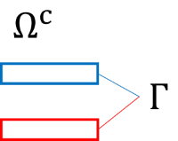
We consider a plate capacitor problem and solve it with a BEM. The setting and notation looks like this:

\( \left\{ \begin{array}{rcl l} - \Delta u &=& 0, \quad &\mathrm{in} \; \Omega^c \,, \\[1ex] \gamma_0 u &=& m\,, & \mathrm{on}\;\Gamma\,, \\[1ex] \lim\limits_{|x| \to \infty} u(x) &=& \mathcal O\left( \displaystyle{ \frac{1}{|x|} }\right)\,, & |x|\to \infty \,. \end{array} \right. \quad\quad\quad\)

largebox = Box ((-2,-2,-2), (2,2,2) )
b1 = Box ( (-1,-1,0.5), (1,1,1) )
b2 = Box ( (-1,-1,-1), (1,1,-0.5))

largebox.faces.name = "outer" 
b1.faces.name = "top" # part of Gamma
b2.faces.name = "bot" # part of Gamma
b1.edges.hpref = 1
b2.edges.hpref = 1
shell = largebox-b1-b2 # Omega^c 
shape = Compound([b1,b2])
mesh = Mesh(OCCGeometry(shape).GenerateMesh(maxh=1))
Draw (mesh);

order = 3
fesH1 = H1(mesh, order=order, definedon=mesh.Boundaries(".*")) 
uH1,vH1 = fesH1.TnT()
fesL2 = SurfaceL2(mesh, order=order-1, dual_mapping=True) 
u,v = fesL2.TnT()
print ("L2-ndof = ", fesL2.ndof, "LH1-ndof = ", fesH1.ndof)

L2-ndof =  576 LH1-ndof =  437

utop = GridFunction(fesH1)
utop.Interpolate(1, definedon=mesh.Boundaries("top"))
ubot = GridFunction(fesH1)
ubot.Interpolate(-1, definedon=mesh.Boundaries("bot"))
m = utop.vec + ubot.vec
Draw (utop + ubot, mesh, draw_vol=False, order=3)

BaseWebGuiScene

Compute boundary integral operators and the mass matrix for right hand side. Solve the linear system of equations:

j = GridFunction(fesL2)
with TaskManager():
    SLPotential = LaplaceSL(u*ds(bonus_intorder=3))
    DLPotential = LaplaceDL(uH1*ds(bonus_intorder=3))
    V = SLPotential*v*ds(bonus_intorder=3)
    K = DLPotential*v*ds(bonus_intorder=3)
    M = BilinearForm(uH1*v*ds(bonus_intorder=3)).Assemble()

with TaskManager():
    pre = BilinearForm(u.Trace()*v.Trace()*ds, diagonal=True).Assemble().mat.Inverse()
    rhs = ((-0.5 * M.mat + K.mat) * m).Evaluate()
    CG(mat = V.mat, pre=pre, rhs = rhs, sol=j.vec, tol=1e-8, 
       maxsteps=200, initialize=False, printrates=False)

Draw (j, mesh, draw_vol=False, order=3);

Evaluation of the Solution

screen = WorkPlane(Axes((0,0,0), X, Z)).RectangleC(4, 4).Face() - Box((-1.1,-1.1,0.4), (1.1,1.1,1.1)) - Box((-1.1,-1.1,-1.1), (1.1,1.1,-0.4))
mesh_screen = Mesh(OCCGeometry(screen).GenerateMesh(maxh=0.25)).Curve(1)
fes_screen = H1(mesh_screen, order=3)
gf_screen = GridFunction(fes_screen)
print ("ndofscreen=", fes_screen.ndof)
with TaskManager():
    gf_screen.Set(-SLPotential(j)+DLPotential(utop)+DLPotential(ubot), 
                  definedon=mesh_screen.Boundaries(".*"), dual=False)
ea = {"euler_angles": (0,90,180)}    
Draw (gf_screen, **ea)

ndofscreen= 2210

BaseWebGuiScene

Compare BEM solution with FEM

Solve the FEM variational formulation with given Dirichlet conditions on the plates and on the ficticious box:

• boundary conditions on the ficticous box given by the Dirichlet trace of the BEM solution

• resolve geometric singularities by anisotropic refinement

mesh_shell = Mesh(OCCGeometry(shell).GenerateMesh(maxh=0.5)).Curve(1)
mesh_shell.RefineHP(2)
fes_shell = H1(mesh_shell, order=3)
gf_shell = GridFunction(fes_shell)
with TaskManager():
    gf_shell.Set(-SLPotential(j)+DLPotential(utop)+DLPotential(ubot), 
                 definedon=mesh_shell.Boundaries("outer"), dual=False)
Draw(gf_shell)

BaseWebGuiScene

fesH1d = H1(mesh_shell, order=order, dirichlet="outer|top|bot")
ud,vd = fesH1d.TnT()
ad = BilinearForm(grad(ud)*grad(vd)*dx).Assemble()
fd = LinearForm(fesH1d).Assemble()
gfud = GridFunction(fesH1d)

utop = GridFunction(fesH1d)
utop.Interpolate(1, definedon=mesh_shell.Boundaries("top"))
ubot = GridFunction(fesH1d)
ubot.Interpolate(-1, definedon=mesh_shell.Boundaries("bot"))

Have a look at the FEM solution:

r = fd.vec - ad.mat * (gf_shell.vec + utop.vec + ubot.vec)
gfud.vec.data = gf_shell.vec + utop.vec + ubot.vec
gfud.vec.data += ad.mat.Inverse(freedofs=fesH1d.FreeDofs()) * r
ea = {"euler_angles": (-90,0,0)}
Draw(gfud, clipping={"y":1, "z":0, "dist":0, 
                     "function" : True }, **ea);

Have a look at the FEM solution (projected on the screen):

gf = GridFunction(fes_screen)
gf.Set(gfud, definedon=mesh_screen.Boundaries(".*"), dual=False)
ea = {"euler_angles": (0,90,180)}
Draw(gf, screen, **ea)

BaseWebGuiScene

Have a look at the error between BEM and FEM solution on the screen:

gf = GridFunction(fes_screen)
gf.Set(gfud - gf_screen, definedon=mesh_screen.Boundaries(".*"), dual=False)
ea = {"euler_angles": (0,90,180)}
Draw(gf, screen, **ea)

BaseWebGuiScene