from ngsolve import *
from netgen.occ import *
import netgen.meshing as meshing
from ngsolve.krylovspace import CG, GMRes
from ngsolve.webgui import Draw
from ngsolve.bem import *
keys: exterior bvp, transmission problem, FEM-BEM coupling, capacitor, electrostatics
Laplace FEM-BEM Coupling#
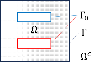
We consider a plate capacitor problem and solve it with a FEM-BEM coupling.
\(\begin{array}{r rcl l} \textnormal{FEM domain}: & - \Delta u &=& 0, \quad &\Omega \,, \\[1ex] \textnormal{BEM domain}: & - \Delta u &=& 0, \quad&\Omega^c\,,\\[1ex] \textnormal{Dirichlet condition}: & \gamma_0 u &=& F_\Gamma & \Gamma_0\,, \\[1ex] \textnormal{coupling condition}: & [ \gamma_0 u] &=& 0 & \Gamma\,, \\[1ex] \textnormal{coupling condition}: & [ \gamma_1 u ] &=& 0 & \Gamma\,, \\[1ex] \textnormal{radiation condition}: & \lim\limits_{|x| \to \infty} u(x) &=& \mathcal O\left( \displaystyle{ \frac{1}{|x|} }\right)\,.\end{array}\quad\quad\quad\) |
|
largebox = Box ((-2,-2,-2), (2,2,2) )
eltop = Box ( (-1,-1,0.5), (1,1,1) )
elbot = Box ( (-1,-1,-1), (1,1,-0.5))

largebox.faces.name = "outer" # coupling boundary
eltop.faces.name = "topface" # Dirichlet boundary
elbot.faces.name = "botface" # Dirichlet boundary
eltop.faces.maxh=0.3
elbot.faces.maxh=0.3

shell = largebox-eltop-elbot # FEM domain
shell.solids.name = "air"

mesh = shell.GenerateMesh(maxh=1)
# mesh.RefineHP(2)
ea = { "euler_angles" : (-67, 0, 110) }
Draw (mesh, clipping={"x":1, "y":0, "z":0, "dist" : 1.1}, **ea);
The coupling needs finite elements in the product space \(H^1(\Omega)\times H^{-\frac12}(\Gamma)\) where \(H^1(\Omega)\) discretise the solution inside the FEM domain \(\Omega\) and \(H^{-\frac12}(\Gamma)\) is needed to resolve the unknown Neumann trace of \(u\) on the coupling boundary \(\Gamma\).
order = 2
fesH1 = H1(mesh, order=order, dirichlet="topface|botface")
fesL2 = SurfaceL2(mesh, order=order-1, dual_mapping=True, definedon=mesh.Boundaries("outer"))
fes = fesH1 * fesL2
fes.ndof
8030
u,dudn = fes.TrialFunction()
v,dvdn = fes.TestFunction()
Set the given Dirichlet boundary conditions on the surfaces of the plates:
gfFGamma = GridFunction(fes)
gfFGamma.components[0].Set ( mesh.BoundaryCF( { "topface" : 1, "botface" : -1 }), BND)
FEM-BEM-Coupling
In the exterior domain \(\Omega^+\) the following representation formula for the solution \(u\) holds:
Within the weak formulation of the interior boundary value problem the transmission boundary conditions are incorporated leading to the FEM-BEM formulation (details below):
A = BilinearForm(grad(u)*grad(v)*dx, check_unused=False).Assemble() # FEM in Omega
F = LinearForm(fes).Assemble()
with TaskManager():
    V = LaplaceSL(dudn*ds("outer"))*dvdn*ds("outer", bonus_intorder=12)
    K = LaplaceDL(u*ds("outer"))*dvdn*ds("outer", bonus_intorder=12)
    D = LaplaceSL(curl(u)*ds("outer"))*curl(v)*ds("outer", bonus_intorder=12)
    M = BilinearForm(u*dvdn*ds("outer"), check_unused=False).Assemble()
Note all matrix contriubutions are build with respect to the number of dofs in the product space where only the relevant entries. This means for instance that
\(A\) is of size \(\verb-fes.ndof x fes.ndof-\) and only \(\verb-H1fes x H1fes-\) dofs are filled.
\(V\) is of size \(\verb-fes.ndof x fes.ndof-\) and only \(\verb-(H1fes bndry dofs) x (H1fes bndry dofs)-\) dofs are filled.
\(K\) is of size \(\verb-fes.ndof x fes.ndof-\) and only \(\verb-fesL2 x (H1fes bndry dofs)-\) dofs are filled.
Due to the product space structure the variational formulation translates such as given by its formula:
lhs = A.mat+D.mat - (0.5*M.mat+K.mat).T - (0.5*M.mat+K.mat) - V.mat
rhs = (F.vec - A.mat * gfFGamma.vec).Evaluate()
Compute the solution of the coupled system (symmetric version) and look at the solution:
bfpre = BilinearForm(grad(u)*grad(v)*dx+1e-10*u*v*dx  + dudn*dvdn*ds("outer") ).Assemble()
pre = bfpre.mat.Inverse(freedofs=fes.FreeDofs(), inverse="sparsecholesky")
with TaskManager():
    sol_sym = CG(mat=lhs, rhs=rhs, pre=pre, tol=1e-8,
                 maxsteps=400, printrates=False)
gfu = GridFunction(fes)
gfu.vec[:] = sol_sym + gfFGamma.vec
Draw(gfu.components[1], clipping={"x" : 1, "y":0, "z":0,
                                  "dist":0.0, "function" : True },
     **ea, order=2);
Details
In the exterior domain \(\Omega^+\) the following representation formula for the solution \(u\) holds:
and the unique traces of \(u\) are related by the Calderon projector
The weak formulation of the interior boundary value problem reads
The coupling condition \([\gamma_1 u]=0\) is now implicitly build in and we used the second equation of the Calderon projector. Adding the first equation of the Calderon projector is known as symmetric coupling formulation. (Note: without the substitution we obtain the Nedelec coupling. The Nedelec coupling is not symmetric.)
References:
Principles of boundary element methods (symmetric coupling)