Maxwell Mixed Conditions

from netgen.occ import *
import netgen.meshing as meshing
from ngsolve import *
from ngsolve.webgui import Draw
from ngsolve.bem import *
from ngsolve import Projector, Preconditioner
from ngsolve.krylovspace import CG, GMRes

keys: PEC Scattering with mixed conditions, Calderon projector, Dirichlet data, Neumann data

Maxwell Mixed Conditions#

Consider the mixed problem:

\( \begin{array}{l rcl r} & \mathrm{curl}\,\mathrm{curl} \boldsymbol E - \kappa^2 \boldsymbol E &=& \boldsymbol 0 &\mathrm{in}\; \Omega^c \,,\\ \textnormal{Dirichlet condition} & \gamma_R \boldsymbol E &=& \boldsymbol m & \mathrm{on}\; \Gamma_0\,,\\ \textnormal{Neumann condition} & \gamma_N \boldsymbol E &=& \boldsymbol j & \mathrm{on}\; \Gamma_1\,, \\ \textnormal{radiation condition} & | \mathrm{curl}\boldsymbol E \times \dfrac{x}{|x|} - i \omega\epsilon \boldsymbol E(x)| &=& \mathcal O(1/|x|^2), & |x|\to \infty\,. \end{array} \quad\quad\quad\)

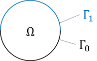
lower half sphere: Dirichlet boundary with given \(\gamma_D \, E = \boldsymbol m\)
upper half sphere: Neumann boundary with given \(\gamma_N \, E = \boldsymbol j\)

NGSolve solution

Define geometry and mesh:

topsphere = Sphere((0,0,0), 1) * Box((-1,-1,0),(1,1,1))
botsphere = Sphere((0,0,0), 1) - Box((-1,-1,0),(1,1,1))
topsphere.faces.name = "neumann" # 1/kappa n x curl E
botsphere.faces.name = "dirichlet" # nxE
shape = Fuse( [topsphere,botsphere] )

h = 0.5
order = 3
mesh = Mesh( OCCGeometry(shape).GenerateMesh(maxh=h, perfstepsend=meshing.MeshingStep.MESHSURFACE)).Curve(order)
Draw (mesh);

Define a manufactured solution \(\boldsymbol E\):

# manufactured solution: kernel with source in point s and direction e
kappa = 1. / h
s = CF((0., 0., 0.))
e = (1.192, -0.189, 2.745)
e = CF(e) / sqrt(e[0] ** 2 + e[1] ** 2 + e[2] ** 2)
xms = CF((x, y , z)) - s
r = Norm(xms)
f = (-kappa ** 2 * r ** 2 - 1j * kappa * r + 1.) / r ** 3
g = (e * xms) * (-kappa ** 2 * r ** 2 - 3. * 1j * kappa * r + 3.) / r ** 5
E = exp(1j * kappa * r) * (f * e - g * xms)
curlE = CF((E[2].Diff(y) - E[1].Diff(z), E[0].Diff(z) - E[2].Diff(x), E[1].Diff(x) - E[0].Diff(y)))

print("kappa = ", kappa)

kappa =  2.0

Boundary Integral Equations

The Calderon projector relates the Dirichlet and the Neumann traces of the solution \(u\), i.e.,

\[\begin{split} \left( \begin{array}{c} \gamma_D E \\ \gamma_N E \end{array}\right) = \left( \begin{array}{cc} V & \frac12 - K \\ \frac12 + K^\intercal & D \end{array} \right) \left( \begin{array}{c} \gamma_N E \\ \gamma_D E \end{array}\right)\,, \end{split}\]

and we use it to solve for the Dirchlet trace on \(\Gamma_1\) and the Neumann trace on \(\Gamma_0\).

Define the finite element product space with \(H^{-\frac12}(\mathrm{curl}_\Gamma, \Gamma)\) and \(H^{-\frac12}(\mathrm{div}_\Gamma, \Gamma)\) conforming finte elements:

order = 3
fesHDiv = HDivSurface(mesh, order=order, complex=True, dirichlet="neumann")
fesHCurl = HCurl(mesh, order=order, complex=True, dirichlet="dirichlet")
fes = fesHCurl * fesHDiv
(uHCurl,uHDiv),(vHCurl,vHDiv) = fes.TnT() 

Get the Dirichlet trace \(\boldsymbol m\) and exact Neumann data \(\boldsymbol j\) as grid functions defined everywhere on \(\Gamma\):

n = specialcf.normal(3)
mjexa = GridFunction(fes)
mj = GridFunction(fes)
mjexa.components[0].Set( Cross( Cross(n, E), n) , 
                        definedon=mesh.Boundaries(".*"), 
                        dual=True) # Hcurl, gamma_R = (nxE)xn
mjexa.components[1].Set( 1/kappa*Cross(n,curlE) , 
                        definedon=mesh.Boundaries(".*"), 
                        dual=True) # Hdiv, gamma_N = 1/k nx curl E

Define Dirichlet boundary condition on the lower half sphere \(\Gamma_0\) and have a look at it:

mj.components[0].Set( mjexa.components[0], 
                     definedon=mesh.Boundaries("dirichlet"), 
                     dual=True) # given Dirichlet data
Draw (Norm(mj.components[0]), mesh, draw_vol=False, order=3);

Define Neumann boundary condition on the upper half sphere \(\Gamma_1\) and have a look at it:

mj.components[1].Set( mjexa.components[1], 
                     definedon=mesh.Boundaries("neumann"), 
                     dual=True) # given Neumann data
Draw (Norm(mj.components[1]), mesh, draw_vol=False, order=3);

Compute boundary integral operators \(\mathrm{V}\), \(\mathrm{K}\), \(\mathrm{D}\) and the mass matrix \(\mathrm M\)

# M, V, K and D 
intorder = 2 * order + 6
with TaskManager(): 
    M = BilinearForm( uHCurl.Trace() * vHDiv.Trace()* ds(bonus_intorder=3)).Assemble() # <Hcurl, Hdiv>  
    V1 = HelmholtzSL(uHDiv.Trace()*ds(bonus_intorder=6), kappa)*vHDiv.Trace()*ds(bonus_intorder=6)
    V2 = HelmholtzSL(div(uHDiv.Trace())*ds(bonus_intorder=6), kappa)*div(vHDiv.Trace())*ds(bonus_intorder=6)
    V = kappa * V1.mat - 1/kappa * V2.mat
    K = HelmholtzDL(uHCurl.Operator("rotated_trace") * ds(bonus_intorder=6), kappa) * vHDiv.Trace() * ds(bonus_intorder=6)
    D1 = HelmholtzSL(uHCurl.Operator("rotated_trace")*ds(bonus_intorder=6), kappa)*uHCurl.Operator("rotated_trace")*ds(bonus_intorder=6)
    D2 = HelmholtzSL(uHCurl.Operator("surface_curl")*ds(bonus_intorder=6), kappa)*vHCurl.Operator("surface_curl")*ds(bonus_intorder=6)
    D = kappa * D1.mat - 1/kappa * D2.mat

Generate right hand side, block matrix and solve the linear system of equations:

\[\begin{split} \left( \begin{array}{c} \gamma_D E \\ \gamma_N E \end{array}\right) = \left( \begin{array}{cc} V & \frac12 - K \\ \frac12 + K^\intercal & D \end{array} \right) \left( \begin{array}{c} \gamma_N E \\ \gamma_D E \end{array}\right)\,, \end{split}\]

and we use it to solve for the Dirchlet trace on \(\Gamma_1\) and the Neumann trace on \(\Gamma_0\).

with TaskManager():
    lhs = V + K.mat - K.mat.T - D
    rhs = ((0.5 * M.mat - K.mat - V + 0.5 * M.mat.T + K.mat.T + D ) * mj.vec).Evaluate()

fesHDivN = HDivSurface(mesh, order=order, dirichlet="neumann") # Dirichlet nodes free dofs
fesHCurlD = HCurl(mesh, order=order, dirichlet="dirichlet") # Neumann nodes free dofs

bfpre = BilinearForm(uHDiv.Trace() * vHDiv.Trace() *ds + uHCurl.Trace() * vHCurl.Trace() *ds).Assemble()
pre = bfpre.mat.Inverse(freedofs=fes.FreeDofs())
with TaskManager():
    sol = GMRes(A=lhs, b=rhs, pre=pre, maxsteps=3000, tol=1e-8, printrates=False)

Compute the Error

Have a look at Neumann data on \(\Gamma_0\) and compute the \(L_2\)-error:

# compare with exact Dirichlet trace
gf = GridFunction(fes)
gf.vec[:] = sol
gfdiv = gf.components[1]
print ("Neumann error =", sqrt(Integrate(Norm(gfdiv + mj.components[1] - mjexa.components[1])**2, mesh.Boundaries(".*"), BND)))
Draw (Norm(gfdiv), mesh.Boundaries("dirichlet"), order=3);

Neumann error = 0.016204016512597914

Have a look at Dirichlet data on \(\Gamma_1\) and compute the \(L_2\)-error:

# compare with the exact Neuman trace  
gfcurl = gf.components[0]
print ("Dirichlet error =", sqrt(Integrate(Norm(gfcurl +mj.components[0] - mjexa.components[0])**2, mesh.Boundaries(".*"), BND)))
Draw (Norm(gfcurl), mesh.Boundaries("neumann"), draw_vol=False, order=3);

Dirichlet error = 0.028593371004442803

References (theory results):

Boundary Element Methods for Maxwell Transmission Problems in Lipschitz Domains

Note that the Calderon-projector in the referenced paper is slightly different from ours as only trace space \(H^{-\frac12}(\mathrm{div}_\Gamma,\Gamma)\) is used. Theoretical results stay the same.