import netgen.meshing as meshing
import numpy as np
from netgen.occ import *
from ngsolve.la import EigenValues_Preconditioner
from ngsolve import *
from ngsolve.bem import *
from ngsolve.webgui import Draw
from ngsolve.krylovspace import GMRes
import matplotlib.pyplot as plt
keys: low frequency breakdown
Maxwell Stabilized#
It is well known that the numerical schemes which rely on the classical second order equation are not stable when passing to the limit \(\kappa \to 0\). The reason for this is that the Gaussian law, which is implicitly embedded for normal wave numbers, is no longer satisfied. The method that we demonstrate here leads to a system of equations in which the continuity equation is maintained (reference below).
We solve the discretized system
where \(\phi_k, \phi_l \in H^{-\frac12}(\mathrm{div}_\Gamma, \Gamma)\) and \(\nu_l, \nu_k\in H^{-\frac12}(\Gamma)\)
We achieve a stabilization for the low-frequency range at the cost of a larger system of equations. The method we propose is independent of the order of approximation. It is important to note that the stabilized system has a one-dimensional kernel that must be explicitly considered.
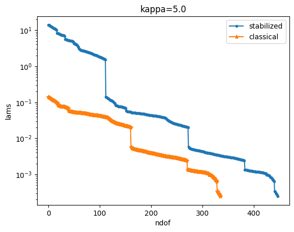
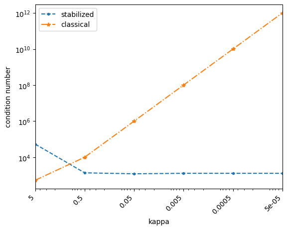
We demonstrate the stabilizing nature of the expanded system by looking at condition numbers for a sequence of wave numbers. We compare the condition number of the stabilized system with the condition number that results from discretization of the classical EFIE equation.
def compute_condition_number(mat):
    """Compute condition number via SVD."""
    s = np.linalg.svd(mat.ToDense(), compute_uv=False)
    s_nonzero = s[s > 1e-14 * s[0]]
    return (s_nonzero[0] / s_nonzero[-2], s) # exclude the one dimensional kernel
def solve_stabilized(mesh, kappa, order=1, intorder=4, use_fmm=True):
    fes_hdiv = HDivSurface(mesh, order=order, complex=True)
    fes_l2 = SurfaceL2(mesh, order=order-1, complex=True, dual_mapping=True)
    fes = fes_hdiv * fes_l2
    (uHDiv, uL2), (vHDiv, vL2) = fes.TnT()
    E_inc = CF((1, 0, 0)) * exp(-1j * kappa * z)

    with TaskManager():
        A_kappa = HelmholtzSL( uHDiv.Trace()*ds(bonus_intorder=intorder) , kappa, use_fmm=use_fmm) * vHDiv.Trace() * ds(bonus_intorder=intorder)
        V_kappa = HelmholtzSL( uL2 * ds(bonus_intorder=intorder) , kappa, use_fmm=use_fmm) * vL2 * ds(bonus_intorder=intorder)
        Q_kappa = HelmholtzSL( div(uHDiv.Trace())*ds(bonus_intorder=intorder) , kappa, use_fmm=use_fmm) * vL2 * ds(bonus_intorder=intorder)

        rhs = LinearForm(E_inc * vHDiv.Trace() * ds(bonus_intorder=2*intorder)).Assemble()
        lhs = A_kappa.mat + Q_kappa.mat + Q_kappa.mat.T + kappa * kappa * V_kappa.mat
        preBlock = BilinearForm( uHDiv.Trace() * vHDiv.Trace() * ds + uL2 * vL2 * ds).Assemble().mat.Inverse(freedofs=fes.FreeDofs())
        sol = GMRes(A=lhs, b=rhs.vec, pre=preBlock, maxsteps=3000, tol=1e-8, printrates=False)

    return lhs, sol, fes, None
def solve_classical(mesh, kappa, order=1, intorder=4, use_fmm=True):
    fes = HDivSurface(mesh, order=order, complex=True)
    u, v = fes.TnT()
    E_inc = CF((1, 0, 0)) * exp(-1j * kappa * z)
    rhs = LinearForm(E_inc * v.Trace() * ds(bonus_intorder=10)).Assemble()
    j = GridFunction(fes)

    with TaskManager():
        V1 = HelmholtzSL( u.Trace()*ds(bonus_intorder=intorder) , kappa, use_fmm=use_fmm) * v.Trace() * ds(bonus_intorder=intorder)
        V2 = HelmholtzSL( div(u.Trace()) * ds(bonus_intorder=intorder), kappa, use_fmm=use_fmm) * div(v.Trace()) * ds(bonus_intorder=intorder)
        V = V1.mat - 1/(kappa**2) * V2.mat
        pre = BilinearForm(u.Trace() * v.Trace() * ds).Assemble().mat.Inverse(freedofs=fes.FreeDofs())
        success = GMRes(A=V, pre=pre, b=rhs.vec, x=j.vec, tol=1e-10, maxsteps=500, printrates=False)

    return V, j, fes, success
def test_low_frequency_stability():
    radius = 1
    sp = Sphere((0, 0, 0), radius)
    mesh = Mesh(OCCGeometry(sp).GenerateMesh(maxh=1, perfstepsend=meshing.MeshingStep.MESHSURFACE)).Curve(4)

    order = 1
    intorder = 4
    use_fmm=False

    kappa_values = [5.0, 0.5, 0.05, 0.005, 0.0005, 0.00005]
    results_stabilized = []
    results_classical = []

    for kappa in kappa_values:
        try:
            A_mat, sol, fes, _ = solve_stabilized(mesh, kappa, order, intorder, use_fmm)
            cond, lams = compute_condition_number(A_mat)
            results_stabilized.append((kappa, A_mat, sol, fes, cond, mesh, cond, lams))

            A_mat, j, fes, success = solve_classical(mesh, kappa, order, intorder, use_fmm)
            cond, lams = compute_condition_number(A_mat)
            results_classical.append((kappa, A_mat, j, fes, mesh, success, cond, lams))

        except Exception as e:
            print("{:10.4f} | Error: {}".format(kappa, e))

    return results_stabilized, results_classical
results_stabilized, results_classical = test_low_frequency_stability()
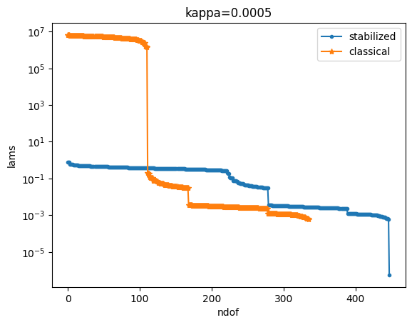
Comparison of the eigenvalue distribution#
def plot_lams(lams_stab, lams_class, title):
    plt.plot(lams_stab, label="stabilized", marker=".")
    plt.plot(lams_class, label="classical", marker="*")
    plt.yscale("log")
    plt.legend()
    plt.xlabel("ndof")
    plt.ylabel("lams")
    plt.title(title)
    plt.show()

prev_cond_stab = None
prev_cond_class = None

for i, ((k_stab, *_, cond_stab, lams_stab), (k_class, *_, cond_class, lams_class)) in enumerate(zip(results_stabilized, results_classical)):
    print(f"kappa: {k_stab}")
    if i == 0:
        print(f"stabilized: cond = {round(cond_stab,3)}")
        print(f"classical: cond = {round(cond_class,3)}")

    if prev_cond_stab is not None:
        print(f"stabilized: ratio = {round(cond_stab/prev_cond_stab,3)}, cond = {round(cond_stab,3)}, prev_cond = {round(prev_cond_stab,3)}")
        print(f"classical: ratio = {round(cond_class/prev_cond_class,3)}, cond = {round(cond_class,3)}, prev_cond = {round(prev_cond_class,3)}")

    plot_lams(lams_stab, lams_class, title=f"kappa={k_stab}")

    prev_cond_stab = cond_stab
    prev_cond_class = cond_class
kappa: 5.0
stabilized: cond = 53353.268
classical: cond = 533.62
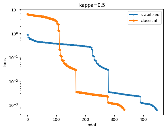
kappa: 0.5
stabilized: ratio = 0.026, cond = 1369.86, prev_cond = 53353.268
classical: ratio = 18.933, cond = 10103.077, prev_cond = 533.62
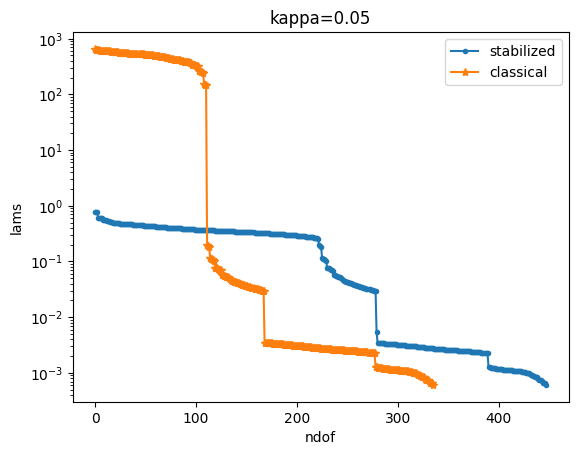
kappa: 0.05
stabilized: ratio = 0.886, cond = 1214.124, prev_cond = 1369.86
classical: ratio = 100.193, cond = 1012254.071, prev_cond = 10103.077
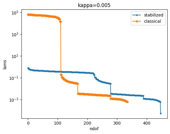
kappa: 0.005
stabilized: ratio = 1.061, cond = 1288.441, prev_cond = 1214.124
classical: ratio = 100.002, cond = 101227364.26, prev_cond = 1012254.071
kappa: 0.0005
stabilized: ratio = 1.0, cond = 1288.426, prev_cond = 1288.441
classical: ratio = 100.0, cond = 10122738432.521, prev_cond = 101227364.26
kappa: 5e-05
stabilized: ratio = 1.0, cond = 1288.426, prev_cond = 1288.426
classical: ratio = 100.0, cond = 1012274414648.184, prev_cond = 10122738432.521
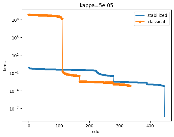
We notice that the condition number of the classical solution grows with \(O(\kappa^{-2})\) whilst the condition number of the stabilized formulation stays constant.
Stability of system matrices#
kappas_stabilized = []
condition_numbers_stabilized = []
kappas_classical = []
condition_numbers_classical = []
for (rs, rc) in zip(results_stabilized, results_classical):
    kappas_stabilized.append(rs[0])
    condition_numbers_stabilized.append(rs[6])
    kappas_classical.append(rc[0])
    condition_numbers_classical.append(rc[6])
plt.xlim(max(kappas_stabilized), min(kappas_stabilized))
plt.loglog(kappas_stabilized, condition_numbers_stabilized, "--", marker=".", label="stabilized")
plt.loglog(kappas_classical, condition_numbers_classical, "-.", marker="*", label="classical")
xs = np.unique(np.r_[kappas_stabilized, kappas_classical])
plt.xticks(xs, [f"{x:g}" for x in xs], rotation=45, ha="right")
plt.legend()
plt.xlabel("kappa")
plt.ylabel("condition number")
plt.show()
Error of solutions#
for (rs, rc) in zip(results_stabilized, results_classical):
    gfs = GridFunction(rs[3])
    sols = rs[2]
    solc = rc[2]
    gfs.vec.data[:] = sols
    kappa = rs[0]
    mesh = rs[5]
    print(f"{kappa=}")
    Draw(gfs.components[0]-solc, mesh)
kappa=5.0
kappa=0.5
kappa=0.05
kappa=0.005
kappa=0.0005
kappa=5e-05
References (theoretical and numerical results):