from ngsolve import *
from netgen.occ import *
from ngsolve.krylovspace import CG, GMRes
from ngsolve.webgui import Draw
from ngsolve.bem import *

keys: homogeneous Laplace bvp with mixed conditions, Calderon projector, Dirichlet data, Neumann data

Laplace with Mixed Conditions

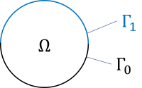
We consider an interior boundary value problem with mixed boundary conditions like this:

\( \left\{ \begin{array}{r rcl r} & \Delta u &=& 0 &\mathrm{in}\; \Omega\,,\\ \textnormal{Dirichlet condition} & \gamma_0 u &=& m & \mathrm{on}\; \Gamma_0\,,\\ \textnormal{Neumann condition} & \gamma_1 u &=& j & \mathrm{on}\; \Gamma_1\,. \end{array} \right. \quad\quad\quad\)

The following representation formula for the solution \(u\) holds:

\[ x \in \Omega: \quad u(x) = \displaystyle{ \int\limits_\Gamma} \displaystyle{\frac{1}{4\,\pi}\, \frac{1}{\| x-y\|} } \, \gamma_1 u (y)\, \mathrm{d} s_y - \displaystyle{ \int\limits_\Gamma} \displaystyle{\frac{1}{4\,\pi}\, \frac{\langle n(y) , x-y\rangle }{\| x-y\|^3} } \, \gamma_0 u (y)\, \mathrm{d} s_y\,. \]

Define the geometry and the mesh:

topsphere = Sphere((0,0,0), 1) * Box((-1,-1,0),(1,1,1))
botsphere = Sphere((0,0,0), 1) - Box((-1,-1,0),(1,1,1))
topsphere.faces.name = "neumann"
botsphere.faces.name = "dirichlet"
shape = Fuse( [topsphere,botsphere] )

order = 3
mesh = Mesh(OCCGeometry(shape).GenerateMesh(maxh=0.25)).Curve(order)
Draw (mesh);

Define the finite element product space \(H^{\frac12}(\Gamma)\times H^{-\frac12}(\Gamma)\) with \(H^{\frac12}(\Gamma)\) conforming elements for the Dirichlet and \(H^{-\frac12}(\Gamma)\) for the Neumann trace.

# use L2 conform elements for the Neumann trace, label all dofs where Neumann data is given:
fesL2 = SurfaceL2(mesh, order=order-1, dirichlet="neumann")
# use H1 conform elements for the Dirichlet trace, label all dofs where Dirichlet data is given:
fesH1 = H1(mesh, order=order, dirichlet="dirichlet", definedon=mesh.Boundaries(".*"))

fes = fesH1 * fesL2
fes.ndof

uH1,uL2 = fes.TrialFunction()
vH1,vL2 = fes.TestFunction()

print ("ndofL2 = ", fesL2.ndof, "ndofH1 = ", fesH1.ndof, "ndof fes =", fes.ndof)

ndofL2 =  2736 ndofH1 =  2116 ndof fes = 4852

Compute and set the Dirichlet and the Neumann data:

uexa = CF(x)
mj = GridFunction(fes)
mjexa = GridFunction(fes)
mjexa.components[0].Interpolate(uexa, definedon=mesh.Boundaries(".*"))
mj.components[0].Set( mjexa.components[0], definedon=mesh.Boundaries("dirichlet")) # given Dirichlet data m

n = specialcf.normal(3)
gradn_uexa = CF((uexa.Diff(x), uexa.Diff(y), uexa.Diff(z))) * n

mjexa.components[1].Interpolate(gradn_uexa, definedon=mesh.Boundaries(".*"))
mj.components[1].Set( mjexa.components[1], definedon=mesh.Boundaries("neumann")) # given Neumann data j

Draw(mj.components[0], mesh, draw_vol=False);

Boundary Integral Equation

The Calderon projector relates the Dirichlet and the Neumann traces of the solution \(u\), i.e.,

\[\begin{split} \left( \begin{array}{c} \gamma_0 u \\ \gamma_1 u \end{array}\right) = \left( \begin{array}{cc} V & \frac12 - K \\ \frac12 + K^\intercal & D \end{array} \right) \left( \begin{array}{c} \gamma_1 u \\ \gamma_0 u \end{array}\right)\,, \end{split}\]

and we use it to solve for the Dirchlet trace on \(\Gamma_1\) and the Neumann trace on \(\Gamma_0\).

Compute boundary integral operators \(\mathrm{V}, \mathrm{K}, \mathrm{D}\) and the mass matrix \(\mathrm{M}\):

eps = 1e-6
intorder = 2 * order + 6
with TaskManager():
    V = LaplaceSL( uL2*ds ) * vL2*ds
    K = LaplaceDL( uH1*ds ) * vL2*ds
    D = LaplaceSL( curl(uH1)*ds ) * curl(vH1)*ds
    M = BilinearForm( uH1 * vL2 * ds(bonus_intorder=3)).Assemble()

Insert all given data in the Dirichlet-to-Neumann map and compute the right hand side vector:

with TaskManager():  
    rhs  = ((0.5 * ( M.mat + M.mat.T) + ( K.mat - K.mat.T) - V.mat - D.mat) * mj.vec).Evaluate()
    lhs = V.mat - K.mat + K.mat.T + D.mat 

Solve for the missing trace data:

with TaskManager():
    pre = BilinearForm( (uH1 * vH1 + uL2 * vL2) * ds(bonus_intorder=3) ).Assemble().mat.Inverse(freedofs=fes.FreeDofs())
    sol = GMRes(A=lhs, b=rhs, pre=pre, tol=1e-8, maxsteps=500, printrates=False)

Have a look at the Neumann data on \(\Gamma_0\) and compute the error:

gf = GridFunction(fes)
gf.vec[:] = sol
gfj = gf.components[1]
print ("Neumann error =", sqrt(Integrate(Norm(gfj + mj.components[1] - mjexa.components[1])**2, mesh.Boundaries(".*"), BND)))
Draw (gfj, mesh.Boundaries("dirichlet"));

Neumann error = 0.00030086008584905217

Have a look at the Dirichlet data on \(\Gamma_1\) and compute the error:

gfm = gf.components[0]
print ("Dirichlet error =", sqrt(Integrate(Norm(gfm + mj.components[0] - mjexa.components[0])**2, mesh.Boundaries(".*"), BND)))
Draw (gfm, mesh.Boundaries("neumann"));

Dirichlet error = 7.886510364731268e-06

Evaluation of the Solution

screen = WorkPlane(Axes((0,0,0), Z, X)).RectangleC(0.5,0.5).Face()
screen.faces.name="screen"
mesh_screen = Mesh(OCCGeometry(screen).GenerateMesh(maxh=0.1)).Curve(1)
fes_screen = H1(mesh_screen, order=13)
gf_screen = GridFunction(fes_screen)
SLPotential = LaplaceSL(uL2*ds(bonus_intorder=intorder))
DLPotential = LaplaceDL(uH1*ds(bonus_intorder=intorder))
repformula = SLPotential(gf) - DLPotential(gf) + SLPotential(mj) - DLPotential(mj)
with TaskManager():
    gf_screen.Set(repformula, definedon=mesh_screen.Boundaries("screen"), dual=False)

Draw(gf_screen)

BaseWebGuiScene