Maxwell Demo 1

keys: exterior Dirichlet bvp, Maxwell single layer potential, EFIE, PEC scattering

from netgen.occ import *
import netgen.meshing as meshing
from ngsolve import *
from ngsolve.webgui import Draw
from ngbem import *
from ngsolve import Projector, Preconditioner
from ngsolve.krylovspace import CG

Loading ngbem library

Dirichlet Boundary Value Problem		Maxwell Single Layer Potential		Variational Formulation
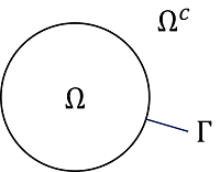
\( \left\{ \begin{array}{rcl l} \mathbf{curl} \, \mathbf{curl}\, \boldsymbol E - \kappa^2 \, \boldsymbol E &=& \boldsymbol 0, \quad &\textnormal{in } \Omega^c \subset \mathbb R^3\,,\\ \gamma_R \,\boldsymbol E &=& \boldsymbol m, \quad & \textnormal{on }\Gamma \\ \left| \mathbf{curl} \, \boldsymbol E( x) - i\,\omega\,\epsilon \, \boldsymbol E( x)\right| &=& \mathcal O\left( \displaystyle \frac{1}{| x|^2}\right), &\textnormal{for} \; |x| \to \infty\,.\end{array} \right. \)	\(\quad \Rightarrow \quad\)	\( \boldsymbol E(x) = \mathrm{SL}(j) \)	\(\quad \Rightarrow \quad\)	\(\left\langle \,\mathrm{SL} (\boldsymbol j),\, \boldsymbol v \right\rangle_{-\frac12} = \left\langle \boldsymbol m , \boldsymbol v\right\rangle_{-\frac12} \)
				\(\mathrm{V} \, \mathrm{j} = \mathrm{M} \, \mathrm{m} \)

NG-BEM Python interface	symbol	FE trial space	FE test space
MaxwellSingleLayerPotentialOperator	\(\mathrm V\)	HDivSurface	HDivSurface
MaxwellDoubleLayerPotentialOperator	\(\mathrm K\)	\(\gamma_R\) HCurl	HDivSurface
MaxwellSingleLayerPotentialOperatorCurl	\(\mathrm D\)	\(\gamma_R\) HCurl	\(\gamma_R\) HCurl
MaxwellDoublelayerPotentialOperator	\(\mathrm K'\)	HDivSurface	\(\gamma_R\) HCurl

Mesh

sp = Sphere( (0,0,0), 1)
mesh = Mesh( OCCGeometry(sp).GenerateMesh(maxh=1, perfstepsend=meshing.MeshingStep.MESHSURFACE)).Curve(4)

Trial and Test Functions

fesHCurl = HCurl(mesh, order=3, complex=True)
fesHDiv = HDivSurface(mesh, order=3, complex=True)
uHCurl,vHCurl = fesHCurl.TnT() 
uHDiv,vHDiv = fesHDiv.TnT()

Dirichlet Data

eps0 = 8.854e-12 
mu0 = 4*pi*1e-7
omega = 1.5e9
kappa = omega*sqrt(eps0*mu0)
E_inc = CF((0,1,0))*exp(1j * kappa * x )
n = specialcf.normal(3)
m = - Cross( Cross(n, E_inc), n)
Draw(Norm(m), mesh, draw_vol=False, order=2) ;

Right Hand Side \(\, \mathrm{rhs} = \mathrm{M}\,\mathrm{m}\)

rhs = LinearForm( m * vHDiv.Trace() *ds(bonus_intorder=3) ).Assemble()

System Matrix \( \,\mathrm{V}\)

V = MaxwellSingleLayerPotentialOperator(fesHDiv, kappa, intorder=10, leafsize=40, eta=3., eps=1e-4)

Solve \( \,\mathrm{V} \mathrm j = \mathrm{rhs}\)

j = GridFunction(fesHDiv)
pre = BilinearForm( uHDiv.Trace() * vHDiv.Trace() *ds ).Assemble().mat.Inverse(freedofs=fesHDiv.FreeDofs()) 
with TaskManager(): 
    CG(mat = V.mat, pre=pre, rhs = rhs.vec, sol=j.vec, tol=1e-8, maxsteps=500, initialize=False, printrates=False)
Draw( j, mesh, draw_vol=False, order=3, min=-2, max=2, animate_complex=True);

Evaluate the Scattered Field on Screen

screen = WorkPlane(Axes( (0,0,-3.5), Z, X)).RectangleC(20,20).Face()
mesh_screen = Mesh( OCCGeometry(screen).GenerateMesh(maxh=1)).Curve(1)
fes_screen = HCurl(mesh_screen, order=3, complex=True)
E_screen = GridFunction(fes_screen)
E_screen.Set (V.GetPotential(j)[0:3], definedon=mesh_screen.Boundaries(".*"))
Draw( E_screen, mesh_screen, draw_vol=False, order=3, min=0, max=0.038, animate_complex=True);

Get the Far Field Pattern

screen = Sphere( (0,0,0), 20)
mesh_screen = Mesh( OCCGeometry(screen).GenerateMesh(maxh=1, perfstepsend=meshing.MeshingStep.MESHSURFACE)).Curve(4)
fes_screen = HCurl(mesh_screen, order=3, complex=True)
E_screen = GridFunction(fes_screen)
E_screen.Set (V.GetPotential(j)[0:3], definedon=mesh_screen.Boundaries(".*"))
Draw(kappa*300*Norm(E_screen)*n, mesh_screen, deformation=True);

Note: For details on convergence rates and low frequency stabilisation of the EFIE look here.