FEM-BEM Coupling

FEM-BEM Coupling#

keys: Transmission problem, FEM-BEM coupling, capacitor, electrostatics, exterior bvp

from ngsolve import *
from netgen.occ import *
import netgen.meshing as meshing
from ngsolve.krylovspace import CG, GMRes
from ngsolve.webgui import Draw
from libbem import *

Loading ngbem library

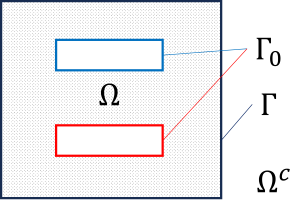
We consider a plate capacitor problem and solve it with a FEM-BEM coupling.


\(\begin{array}{r rcl l} \textnormal{FEM domain}: & - \Delta u &=& 0, \quad &\Omega \,, \\[1ex] \textnormal{BEM domain}: & - \Delta u &=& 0, \quad&\Omega^c\,,\\[1ex] \textnormal{Dirichlet condition}: & \gamma_0 u &=& u_0 & \Gamma_0\,, \\[1ex] \textnormal{coupling condition}: & [ \gamma_0 u] &=& 0 & \Gamma\,, \\[1ex] \textnormal{coupling condition}: & [ \gamma_1 u ] &=& 0 & \Gamma\,, \\[1ex] \textnormal{radiation condition}: & \lim\limits_{\|x\| \to \infty} u(x) &=& \mathcal O\left( \displaystyle{ \frac{1}{\|x\|} }\right)\,.\end{array}\)	\(\quad\quad\quad\)

largebox = Box ((-2,-2,-2), (2,2,2) )
b1 = Box ( (-1,-1,0.5), (1,1,1) )
b2 = Box ( (-1,-1,-1), (1,1,-0.5))

b1.name = "top"
b2.name = "bot"
b1.faces.name = "topface" # Dirichlet boundary
b2.faces.name = "botface" # Dirichlet boundary
b1.faces.maxh=0.3
b2.faces.maxh=0.3
shell = largebox-b1-b2 # FEM domain Omega
shell.name = "air"
largebox.faces.name = "outer" # coupling boundary

shape = shell
mesh = Mesh(OCCGeometry(shape).GenerateMesh(maxh=1))

Draw (mesh, clipping={"x":1, "y":0});

In the exterior domain \(\Omega^+\) the following representation formula for the solution \(u\) holds:

\[ x \in \Omega^c: \quad u(x) = - \int\limits_\Gamma \displaystyle{\frac{1}{4\,\pi}\, \frac{1}{\| x-y\|} } \, \gamma_1 u (y)\, \mathrm{d}\sigma_y + \int\limits_\Gamma \displaystyle{\frac{1}{4\,\pi}\, \frac{\langle n(y) , x-y\rangle }{\| x-y\|^3} } \, \gamma_0 u (y)\, \mathrm{d}\sigma_y\,, \]

and the unique traces of \(u\) are related by the Calderon projector

\[\begin{split} \left( \begin{array}{c} \gamma_0 u \\ \gamma_1 u \end{array}\right) = \left( \begin{array}{cc} -V & \frac12 + K \\ \frac12 - K^\intercal & -D \end{array} \right) \left( \begin{array}{c} \gamma_1 u \\ \gamma_0 u \end{array}\right) \end{split}\]

The weak formulation of the interior boundary value problem reads

\[\begin{split} \begin{array}{r rcl} \forall v \in H^1(\Omega): \quad \quad & \displaystyle { \int\limits_{\Omega}} \langle \nabla u(x), \nabla v(x)\rangle \, \mathrm{d} x - \displaystyle{ \int\limits_{\Gamma} } \gamma_1 u(x) \cdot \gamma_0 v(x) \, \mathrm{d}\sigma &=& \displaystyle{ \int\limits_{\Omega} }f(x) \cdot v(x) \, \mathrm{d} x \\[1ex] \textnormal{substitution of } \gamma_1 u: & \displaystyle { \int\limits_{\Omega}} \langle \nabla u(x), \nabla v(x)\rangle \, \mathrm{d} x - \displaystyle{ \int\limits_{\Gamma} } \left(\left( \frac12 - K^\intercal\right) \,\gamma_1 u - D \, \gamma_0 u\right) \cdot \gamma_0 v(x) \, \mathrm{d}\sigma &=& \displaystyle{ \int\limits_{\Omega} }f(x) \cdot v(x) \, \mathrm{d} x \end{array} \end{split}\]

The coupling condition \([\gamma_1 u]=0\) is now implicitly build in and we used the second equation of the Calderon projector. Adding the first equation of the Calderon projector is known as symmetric coupling formulation. To understand better the structure of the discretized system the dofs are splitted in degrees of freedom inside \(\Omega\) and those on the boundary \(\Gamma\).

\[\begin{split} \left( \begin{array}{ccc } A_{\Omega\Omega} & A_{\Omega\Gamma} & 0 \\ A_{\Gamma\Omega} & A_{\Gamma\Gamma } + D & -\frac12 M^\intercal + K^\intercal \\ 0 & -\frac12 M + K & -V \end{array}\right) = \left( \begin{array}{c} u \\ \gamma_0 u \\ \gamma_1 u \end{array}\right) = \left( \begin{array}{c} F_{\Omega} \\ F_{\Gamma}\\ 0 \end{array}\right) \,. \end{split}\]

Note: without the substitution we obtain the Nedelec coupling. The Nedelec coupling is not symmetric.

Generate the finite element space for \(H^1(\Omega)\) and set the given Dirichlet boundary conditions on the surfaces of the plates:

order = 2
fesH1 = H1(mesh, order=order, dirichlet="topface|botface") # H^1 conforming elements with H^(1/2) conforming elements on boundary
print ("H1-ndof = ", fesH1.ndof)
u,v = fesH1.TnT()
a = BilinearForm(grad(u)*grad(v)*dx).Assemble() # system matrix of variational formulation in Omega
dirtopface = GridFunction(fesH1)
dirbotface = GridFunction(fesH1)
dirtopface.Set(1, definedon=mesh.Boundaries("topface")) # boundary condition on upper plate
dirbotface.Set(-1, definedon=mesh.Boundaries("botface")) # boundary condition on lower plate
r = LinearForm(fesH1).Assemble()
f = r.vec - a.mat * (dirtopface.vec + dirbotface.vec)

H1-ndof =  7373

The finite element space \(\verb-fesH1-\) provides \(H^{\frac12}(\Gamma)\) conforming element to discretize the Dirichlet trace on the coupling boundary \(\Gamma\). However we still need \(H^{-\frac12}(\Gamma)\) conforming elements to discretize the Neumann trace of \(u\) on the coupling boundary. Here it is:

fesL2 = SurfaceL2(mesh, order=order-1, dual_mapping=True, definedon=mesh.Boundaries("outer")) # H^(-1/2) conforming elements
f2 = LinearForm(fesL2).Assemble()  # 0-vector
print ("L2-ndof = ", fesL2.ndof)

L2-ndof =  1450

Generate the the single layer potential \(V\), double layer potential \(K\) and hypersingular operator \(D\):

with TaskManager():
    V = SingleLayerPotentialOperator(fesL2, intorder=12, eps=1e-10, method="aca")
    K = DoubleLayerPotentialOperator(fesH1, fesL2, trial_definedon=mesh.Boundaries("outer"),  test_definedon=mesh.Boundaries("outer"), method="aca", intorder=12, eps=1e-10)
    D = HypersingularOperator(fesH1, definedon=mesh.Boundaries("outer"), intorder=12, eps=1e-10, method="aca")
    M = BilinearForm(fesH1.TrialFunction()*fesL2.TestFunction().Trace()*ds("outer")).Assemble()

trial is definedon: 0: 111111000000000000
test is definedon: 0: 111111000000000000
trial is definedon: 0: 111111000000000000
test is definedon: 0: 111111000000000000

Setup the coupled system matrix and the right hand side:

sym = BlockMatrix ([[a.mat+D.mat, (-0.5*M.mat+K.mat).T], [(-0.5*M.mat+K.mat), -V.mat]])
nonsym = BlockMatrix ([[a.mat, -M.mat.T ], [(-0.5*M.mat+K.mat), -V.mat]])
rhs = BlockVector([f, f2.vec])

l2mass = BilinearForm( fesL2.TrialFunction().Trace()*fesL2.TestFunction().Trace()*ds).Assemble()
astab = BilinearForm((grad(u)*grad(v) + 1e-10 * u * v)*dx).Assemble()
pre = BlockMatrix ([[astab.mat.Inverse(freedofs=fesH1.FreeDofs(), inverse="sparsecholesky"), None], [None, l2mass.mat.Inverse(freedofs=fesL2.FreeDofs())] ])

Compute the solution of the coupled system (symmetric version) and look at the solution:

with TaskManager():
    sol_sym = CG(mat=sym, rhs=rhs, pre=pre, tol=1e-8, maxsteps=400, printrates=False)

gfu = GridFunction(fesH1)
gfu.vec[:] = sol_sym[0] + dirtopface.vec + dirbotface.vec
Draw(gfu, clipping={"y":1, "z":0, "dist":0.0, "function" : True }); # Turn on the Clipping Plane in Control panel!

Compute the solution of the coupled system (non-symmetric version) and look at the solution:

sol_nonsym = GMRes(A=nonsym, b=rhs, pre=pre, tol=1e-8, maxsteps=400, printrates=False)

gfu = GridFunction(fesH1)
gfu.vec[:] = sol_nonsym[0] + dirtopface.vec + dirbotface.vec
Draw(gfu, clipping={"y":1, "z":0, "dist":0.0, "function" : True }, min=-1, max=1);

References:

Principles of boundary element methods (symmetric coupling)

On the Coupling of Boundary Integral and Finite Element Methods (non-symmetric coupling)