BIE for Laplace

Energy Spaces and Trace Spaces

\[\begin{split} \begin{array}{rcccccc} \textnormal{natural sequence:} &H^{\frac12}(\Gamma) & \xrightarrow{\nabla_{\Gamma}} & \boldsymbol{H}^{-\frac12}(\mathrm{curl}_{\Gamma},{\Gamma}) & \xrightarrow{\mathrm{curl}_{\Gamma}}& H^{-\frac12}({\Gamma})& \\[1ex] &\gamma_0 \Big\uparrow && \gamma_R \Big\uparrow && \gamma_{\boldsymbol n} \Big\uparrow &\\[1ex] \textnormal{energy spaces:} &H^1({\Omega}) & \xrightarrow{\nabla} & H(\mathbf{curl},{\Omega}) & \xrightarrow{\mathbf{curl}}& H(\mathrm{div},{\Omega}) & \xrightarrow{\mathrm{div}} \; L_2(\Omega) \\[1ex] &\gamma_0 \Big\downarrow && \gamma_D \Big\downarrow && \gamma_{\boldsymbol n} \Big\downarrow &\\[1ex] \textnormal{dual sequence:} &H^{\frac12}(\Gamma) & \xrightarrow{\mathbf{curl}_{\Gamma}} & \boldsymbol{H}^{-\frac12}(\mathrm{div}_{\Gamma},{\Gamma}) & \xrightarrow{\mathrm{div}_{\Gamma}}& H^{-\frac12}({\Gamma})& \end{array} \end{split}\]

Trace Operators

\[\begin{split} \begin{array}{r rcl } \textnormal{Dirichlet trace:} \; & \gamma_0 u &=& u \\[1ex] \textnormal{Neumann trace} \quad & \gamma_1 u &=& \langle \boldsymbol n, \nabla\, u \rangle \,. \end{array} \end{split}\]

• densities in \( H^{\frac12}\left( \Gamma\right) \) are weakly continous

• densities in \( H^{-\frac12}\left( \Gamma\right) \) are not continous

Layer Potentials

\[\begin{split} \begin{array}{r rcl} \textnormal{single layer potential:} \; \mathrm{SL}\left( j \right) (x) &=& \displaystyle{ \int\limits_\Gamma \displaystyle{\frac{1}{4\,\pi}\, \frac{1}{\| x-y\|} } \, j(y)\, \mathrm{d}\sigma_y } \\ \textnormal{double layer potential:} \; \mathrm{DL}\left(m \right)(x) &=& \displaystyle{ \int\limits_\Gamma \displaystyle{\frac{1}{4\,\pi}\, \frac{ \langle n(y), x-y \rangle }{\| x-y\|^3} } \, m(y)\, \mathrm{d}\sigma_y } \end{array}\end{split}\]

Laplace Dirichlet BVP

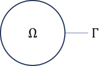
Let \(u\) denote the electrostatic potential that arises under given Dirichlet boundary condition inside a source-free domain \(\Omega \in \mathbb R^3\). Thus, \(u\) solves the interior boundary value problem

\( \left\{ \begin{array}{rcl l} \Delta u &=& 0\,, \quad & \Omega \subset \mathbb R^3\,, \\ \gamma_0 u &=& u_0\,, \quad & \Gamma = \partial \Omega\,. \end{array} \right. \)	\(\quad\quad\quad\)

From here we can choose an direct or an indirect ansatz.

1. Direct Method \(\quad u = \mathrm{SL}(u_1) - \mathrm{DL}(u_0)\)

\[\begin{split} \begin{array}{r rcl } \textnormal{variational formulation } & \forall v\in H^{-\frac12}(\Gamma): \, \big\langle \gamma_0 \left(\mathrm{SL}(u_1)\right), v \big\rangle_{-\frac12} &=& \big\langle u_0, v\big\rangle_{-\frac12} + \big\langle \gamma_0 \left(\mathrm{DL}(u_0)\right), v \big\rangle_{-\frac12} \\ \textnormal{discretisation} & \mathrm{V} \,\mathrm{u}_1 &=& \left( \frac12 \,\mathrm{M} + \mathrm{K} \right) \, \mathrm{u}_0 \\ \end{array}\end{split}\]

2. Indirect Method \(\quad u = \mathrm{SL}(j) \)

\[\begin{split} \begin{array}{r rcl } \textnormal{variational formulation } & \forall v\in H^{-\frac12}(\Gamma): \, \big\langle \gamma_0 \left(\mathrm{SL}(j)\right), v \big\rangle_{-\frac12} &=& \big\langle u_0, v\big\rangle_{-\frac12} \\ \textnormal{discretisation} & \mathrm{V} \, \mathrm{j} &=& \mathrm{M} \,\mathrm{u}_0 \end{array} \end{split}\]

Laplace Neumann BVP

Let \(u\) denote the electrostatic potential that arises under given Neumann boundary condition inside a source-free domain \(\Omega \in \mathbb R^3\). Thus, \(u\) solves the boundary value problem

\( \left\{ \begin{array}{rcl l} \Delta u &=& 0\,, \quad & \Omega \subset \mathbb R^3\,, \\ \gamma_1 u &=& u_1\,, \quad & \Gamma = \partial \Omega\,. \end{array} \right. \)	\(\quad\quad\quad\)

From here we can choose an direct or an indirect ansatz.

1. Direct Method \(\quad u = \mathrm{SL}(u_1) - \mathrm{DL}(u_0)\)

\[\begin{split} \begin{array}{r rcl } \textnormal{variational formulation } & \forall v\in H^{\frac12}(\Gamma): \, \big\langle v, \gamma_1 \left(\mathrm{DL}(u_0)\right) \big\rangle_{-\frac12} &=& \big\langle u_1, v\big\rangle_{-\frac12} - \big\langle v, \gamma_1 \left(\mathrm{SL}(u_1)\right) \big\rangle_{-\frac12} \\ \textnormal{discretisation} & \left( \mathrm{D} + \mathrm{S}\right) \mathrm{u}_0 &=& \left( \frac12 \mathrm{M} - \mathrm{K}^\intercal\right) \, \mathrm{u}_1 \end{array} \end{split}\]

2. Indirect method \(\quad u = \mathrm{DL}(m)\)

\[\begin{split} \begin{array}{r rcl } \textnormal{variational formulation } & \forall \quad v\in H^{\frac12}(\Gamma):\, \big\langle v, \gamma_1 \left(\mathrm{DL}(m)\right) \big\rangle_{-\frac12} &=& \big\langle u_1, v\big\rangle_{-\frac12} \\ \textnormal{discretisation} & \left( \mathrm{D} + S\right) \, \mathrm{m} &=& \mathrm{M}\,\mathrm{u}_1 \end{array} \end{split}\]

NG-BEM Operators

The discretiszation of the boundary integral equations leads to the following layer potential operators:

	trial space	test space
single layer potential operator	\(H^{-\frac12}(\Gamma)\)	\(H^{-\frac12}(\Gamma)\)
double layer potential operator	\(H^{\frac12}(\Gamma)\)	\(H^{-\frac12}(\Gamma)\)
hypersingular operator	\(H^{\frac12}(\Gamma)\)	\(H^{\frac12}(\Gamma)\)
adjoint double layer potential operator	\(H^{-\frac12}(\Gamma)\)	\(H^{\frac12}(\Gamma)\)

• NG-BEM implements the layper potential operators based on conforming finite element spaces.

• The finite element spaces are either natural traces of energy spaces:

  • The trace space \(H^{\frac12}(\Gamma)\) is naturally given by \(\gamma_0\)H1.

  • The trace space \(H^{-\frac12}(\Gamma)\) which is explicitely implemented as finite element (FE) space SurfaceL2.

Python interface	symbol	FE trial space	FE test space
SingleLayerPotentialOperator	\(\mathrm V \)	SurfaceL2	SurfaceL2
DoubleLayerPotentialOperator	\(\mathrm K \)	\(\gamma_0\) H1	SurfaceL2
HypersingularOperator	\(\mathrm D\)	\(\gamma_0\) H1	\(\gamma_0\) H1
DoubleLayerPotentialOperator	\(\mathrm K'\)	SurfaceL2	\(\gamma_0\) H1