Laplace Demo 3

Laplace Demo 3#

keys: exterior Dirichlet bvp, single and double layer potential, evaluate representation formula, plate capacitor

from ngsolve import *
from netgen.occ import *
import netgen.meshing as meshing
from ngsolve.krylovspace import CG, GMRes
from ngsolve.webgui import Draw
from ngbem import *

Loading ngbem library

Dirichlet Boundary Value Problem		Single and Double Layer		Variational Formulation
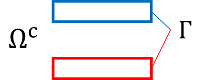
\( \left\{ \begin{array}{rcl l} -\Delta u &=& 0, \quad &\Omega^c \\ \gamma_0 u&=& u_0, \quad &\Gamma \\ \lim\limits_{\|x\| \to \infty} u(x) &=& \mathcal O\left( \displaystyle{ \frac{1}{\|x\|} }\right)\,, & \|x\|\to \infty \end{array} \right. \)	\(\quad \Rightarrow \quad\)	\( u(x) = \mathrm{SL}(u_1) - \mathrm{DL}(u_0) \)	\(\quad \Rightarrow \quad\)	\(\left\langle \gamma_0 \left(\mathrm{SL}(u_1)\right), v \right\rangle_{-\frac12}= \left\langle u_0, v\right\rangle_{-\frac12} + \left\langle \gamma_0 \left(\mathrm{DL}(u_0)\right), v\right\rangle_{-\frac12}\)

				\(\mathrm{V} \, \mathrm{u}_1 = \left( -\frac12 \,\mathrm{M} + \mathrm{K} \right) \, \mathrm{u}_0 \)

NG-BEM Python interface	symbol	FE trial space	FE test space
`SingleLayerPotentialOperator`	\(\mathrm V \)	`SurfaceL2`	`SurfaceL2`
`DoubleLayerPotentialOperator`	\(\mathrm K \)	\(\gamma_0\) `H1`	`SurfaceL2`
`HypersingularOperator`	\(\mathrm D\)	\(\gamma_0\) `H1`	\(\gamma_0\) `H1`
`DoubleLayerPotentialOperator`	\(\mathrm K'\)	`SurfaceL2`	\(\gamma_0\) `H1`

Mesh

largebox = Box ((-2,-2,-2), (2,2,2) )
b1 = Box ( (-1,-1,0.5), (1,1,1) )
b2 = Box ( (-1,-1,-1), (1,1,-0.5))
largebox.faces.name = "outer" 
b1.faces.name = "top" # part of Gamma
b2.faces.name = "bot" # part of Gamma
shell = largebox-b1-b2 # Omega^c 
shape = Compound([b1,b2])
mesh = Mesh(OCCGeometry(shape).GenerateMesh(maxh=1))

Trial and Test Functions

order = 3
fesH1 = H1(mesh, order=order, definedon=mesh.Boundaries(".*")) 
uH1,vH1 = fesH1.TnT()
fesL2 = SurfaceL2(mesh, order=order-1, dual_mapping=True)
u,v = fesL2.TnT()

Dirichlet Data

utop = GridFunction(fesH1)
utop.Interpolate(1, definedon=mesh.Boundaries("top"))
ubot = GridFunction(fesH1)
ubot.Interpolate(-1, definedon=mesh.Boundaries("bot"))
u0 = utop.vec + ubot.vec
Draw (utop + ubot, mesh, draw_vol=False, order=3);

Layer Potential Operators \(\, \mathrm{V}, \; \mathrm{K}\) and Mass Matrix \(\,\mathrm{M}\)

with TaskManager():
    V = SingleLayerPotentialOperator(fesL2, intorder=12, eps=1e-4)
    K = DoubleLayerPotentialOperator(fesH1, fesL2, intorder=12, eps=1e-4)
    M = BilinearForm( uH1.Trace() * v.Trace() * ds(bonus_intorder=3)).Assemble()

Right Hand Side \(\, \mathrm{rhs} = \left( -\frac12\mathrm{M}+\mathrm{K} \right) \mathrm{u}_0\)

rhs = ((-0.5 * M.mat + K.mat) * u0).Evaluate()

Solve \(\, \mathrm{V} \mathrm{u}_1 = \mathrm{rhs} \)

u1 = GridFunction(fesL2)
pre = BilinearForm(u.Trace()*v.Trace()*ds, diagonal=True).Assemble().mat.Inverse()
with TaskManager():
    CG(mat = V.mat, pre=pre, rhs = rhs, sol=u1.vec, tol=1e-8, maxsteps=200, initialize=False, printrates=False)
Draw (u1, mesh, draw_vol=False, order=3);

Evaluate on Screen

screen = WorkPlane(Axes((0,0,0), X, Z)).RectangleC(4, 4).Face() - Box((-1.1,-1.1,0.4), (1.1,1.1,1.1)) - Box((-1.1,-1.1,-1.1), (1.1,1.1,-0.4))
mesh_screen = Mesh(OCCGeometry(screen).GenerateMesh(maxh=0.25)).Curve(1)
fes_screen = H1(mesh_screen, order=3)
gf_screen = GridFunction(fes_screen)
with TaskManager():
    gf_screen.Set(-V.GetPotential(u1)+K.GetPotential(utop)+K.GetPotential(ubot), definedon=mesh_screen.Boundaries(".*"), dual=False)
Draw (gf_screen);