Laplace Demo 1#
keys: homogeneous Dirichlet bvp, single layer potential ansatz, single layer potential operator, electrostatics
from netgen.occ import *
from ngsolve import *
from ngsolve.webgui import Draw
from ngbem import *
from ngsolve import Projector, Preconditioner
from ngsolve.krylovspace import CG
Loading ngbem library
Dirichlet Boundary Value Problem |
Single Layer Potential |
Variational Formulation |
||
|---|---|---|---|---|
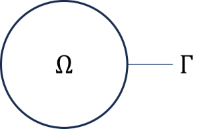
\( \left\{ \begin{array}{rcl l} -\Delta u &=& 0, \quad &\Omega \\ \gamma_0 u&=& u_0, \quad &\Gamma \end{array} \right. \) |
\(\quad \Rightarrow \quad\) |
\( u(x) = \mathrm{SL}(j) \) |
\(\quad \Rightarrow \quad\) |
\(\left\langle \gamma_0 \left(\mathrm{SL}(j)\right), v \right\rangle_{-\frac12} = \left\langle u_0, v\right\rangle_{-\frac12} \) |
|
\(\mathrm{V} \, \mathrm{j} = \mathrm{M} \, \mathrm{u}_0 \) |
NG-BEM Python interface |
symbol |
FE trial space |
FE test space |
|---|---|---|---|
|
\(\mathrm V \) |
|
|
|
\(\mathrm K \) |
\(\gamma_0\) |
|
|
\(\mathrm D\) |
\(\gamma_0\) |
\(\gamma_0\) |
|
\(\mathrm K'\) |
|
\(\gamma_0\) |
Mesh
sp = Sphere( (0,0,0), 1)
mesh = Mesh( OCCGeometry(sp).GenerateMesh(maxh=0.3)).Curve(3)
Draw(mesh);
Trial and Test Functions
fesL2 = SurfaceL2(mesh, order=3, dual_mapping=True)
u,v = fesL2.TnT()
Right Hand Side \(\;\mathrm{M}\mathrm{u}_0\)
u0 = 1/ sqrt( (x-1)**2 + (y-1)**2 + (z-1)**2 )
Mu0 = LinearForm (u0*v.Trace()*ds(bonus_intorder=3)).Assemble()
System Matrix \( \; \mathrm{V}\)
V = SingleLayerPotentialOperator(fesL2, intorder=10, method="aca")
Solve \(\; \mathrm{V}\mathrm{j} = \mathrm{M}\mathrm{u}_0\)
j = GridFunction(fesL2)
pre = BilinearForm(u*v*ds, diagonal=True).Assemble().mat.Inverse()
with TaskManager(pajetrace=1000*1000*1000):
    CG(mat = V.mat, pre=pre, rhs = Mu0.vec, sol=j.vec, tol=1e-8, maxsteps=200, initialize=False, printrates=False)
Draw (j);
Notes:
For details on the analysis of boundary integral equations derived from elliptic partial differential equations, see for instance Strongly Elliptic Systems and Boundary Integral Equations.
In our implementation, the integration of singular pairings is done as proposed in Randelementmethoden